Don Knuth’s MIP, 64 years later

In 1960, the famed computer scientist Don Knuth wrote a technical paper in which he considered an integer programming model for minimizing memory access latency of an IBM 650. I’ve included a screenshot of the 51 variable, 43 constraint problem at the end of this post.

Prof Knuth describes the problem and his attempts to solve it in an unpublished note on his website. Knuth used a technique of Ralph Gomory published the same year, which he somehow became aware of despite the absence of email, the web, arxiv, or large language models. I asked ChatGPT to render an image of Gomory and Knuth pensively sitting atop a mainframe. It refused for privacy reasons. Here is the best it could do:

Knuth ran Gomory’s algorithm on an IBM 650 with less than 10K of memory, but was unable to find an optimal solution. Thirty-five years later (when I was an undergrad), Dimitris Alevras successfully found the optimum value of 22996 using CPLEX on a SPARCstation 5. I am proud to say I have coded on such a machine! Alveras reported that “32,200 branch-and-bound nodes” were needed to solve the problem to optimality. No CPU time is reported in Knuth’s writeup, but we can safely assume the solution time was minutes or likely hours.

I grabbed the problem formulation from Knuth’s writeup and translated it into Python code (copilot was helpful for this purpose). An MPS file with the model can be found here.

I found that the open source solver SCIP was able to find an optimal solution in two tenths of a second, and that Gurobi was able to solve it in less than 0.1s.

This is another testament to the amazingly wonderful effectiveness of operations research!

Creating Equation Haikus using Constraint Programming

Bob Bosch pointed out (in a response to Shea Serrano, wonderfully…) that 77 + 123 = 200 is a haiku in English:

Somewhat related. This is a haiku (when read in English): pic.twitter.com/aeTMPPIUxi

— Robert (Bob) Bosch (@baabbaash) September 19, 2019

How many such haikus are there? Well, we can use constraint satisfaction (CSP) to give us an idea (Python code here for the impatient):

A traditional haiku consists of three lines: the first line has five syllables, the second seven, and the last five, for a total of seventeen syllables.

We can write equations that describe our problem. First, let’s define the function s[n] as the number of syllables in the English words for n. For example, s[874] = 7; try saying “eight hundred seventy four” out loud. It’s not that hard in English to compute s[n]; at least, I don’t think I messed it up.

Let’s call A the number in the first line of the haiku, B the second, and C the third. If we want a haiku with the right number of syllables and for the equation it describes to hold, all we need is:

s[A] = 5
1 + s[B] = 7 (since “plus” is one syllable)
2 + s[C] = 5 (since “equals” is two syllables)
A + B = C

If you let A=77, B=123, C=200 as in Bob’s example, you will see the above equations hold.

Using the constraint package in Python, it’s easy to create this model and solve it. Here is the code. A great thing about CSP solvers is that they will not just give you one of the solutions to the model, but all the solutions, at least for cases where A, B, C <= 9999. It turns out there are 279 such haikus, including

eight thousand nineteen
plus nine hundred eighty one
equals nine thousand

and the equally evocative

one hundred fourteen
plus one hundred eighty six
equals three hundred

Of course, this is not the only possible form for an equation haiku. For example, why not:

A
+ B + C
= D

I invite you to modify the code and find other types of equation haikus!

Optimizing 19th Century Typewriters

The long title for this post is: “Optimizing 19th Century Typewriters using 20th Century Code in the 21st Century”.

Patrick Honner recently shared Hardmath123’s wonderful article “Tuning a Typewriter“. In it, Hardmath123 explores finding the best way to order the letters A-Z on an old and peculiar typewriter. Rather than having a key for each letter as in a modern keyboard, the letters are laid out on a horizontal strip. You shift the strip left or right to find the letter you want, then press a key to enter it:

What’s the best way to arrange the letters on the strip? You probably want to do it in such a way that you have to shift left and right as little as possible. If consecutive letters in the words you’re typing are close together on the strip, you will minimize shifting and type faster.

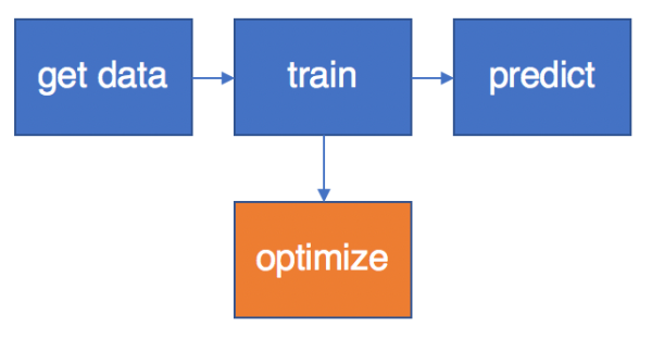
The author’s approach is to:

• Come up with an initial ordering at random,
• Compute the cost of the arrangement by counting how many shifts it takes to type out three well-known books,
• Try to find two letters that when you swap them results in a lower cost,
• Swap them and repeat until you can no longer find an improving swap.

This is a strong approach that leads to the same locally optimal arrangements, even when you start from very different initial orderings. It turns out that this is an instance of a more general optimization problem with an interesting history: quadratic assignment problems. I will explain what those are in a moment.

Each time I want to type a letter, I have to know how far to shift the letter strip. That depends on two factors:

1. The letter that I want to type in next, e.g. if I am trying to type THE and I am on “T”, “H” comes next.
2. The location of the next letter, relative to the current one T. For example, if H is immediately to the left of T, then the location is one shift away.

If I type in a bunch of letters, the total number of shifts can be computed by multiplying two matrices:

• A frequency matrix F. The entry in row R and column C is a count of how often letter R precedes letter C. If I encounter the word “THE” in my test set, then I will add 1 to F(“T”, “H”) and 1 to F(“H”, “E”).
• A distance matrix D. The entry in row X and column Y is the number of shifts between positions X and Y on the letter strip. For example, D(X, X+1) = 1 since position X is next to position X+1.

Since my problem is to assign letters to positions, if I permute the rows and columns of D and multiply this matrix with F, I will get the total number of shifts required. We can easily compute F and D for the typewriter problem:

• To obtain F, we can just count how often one letter follows another and record entries in the 26 x 26 matrix. Here is a heatmap for the matrix using the full Project Gutenberg files for the three test books:

• The distance matrix D is simple: if position 0 is the extreme left of the strip and 25 the extreme right, d_ij = abs(i – j).

The total number of shifts is obtained by summing f_ij * d_p(i),p(j) for all i and j, where letter i is assigned to location p(i).

Our problem boils down to finding a permutation that minimizes this matrix multiplication. Since the cost depends on the product of two matrices, this is referred to as a Quadratic Assignment Problem (QAP). In fact, problems very similar to this one are part of the standard test suite of problems for QAP researchers, called “QAPLIB“. The so-called “bur” problems have similar flow matrices but different distance matrices.

We can use any QAP solution approach we like to try to solve the typewriter problem. Which one should we use? There are two types of approaches:

• Those that lead to provably global optimal solutions,
• Heuristic techniques that often provide good results, but no guarantees on “best”.

QAP is NP-hard, so finding provably optimal solutions is challenging. One approach for finding optimal solutions, called “branch and bound”, boils down to dividing and conquering by making partial assignments, solving less challenging versions of these problems, and pruning away assignments that cannot possibly lead to better solutions. I have written about this topic before. If you like allegories, try this post. If you prefer more details, try my PhD thesis.

The typewriter problem is size 26, which counts as “big” in the world of QAP. Around 20 years ago I wrote a very capable QAP solver, so I recompiled it and ran it on this problem – but didn’t let it finish. I am pretty sure it would take at least a day of CPU time to solve, and perhaps more. It would be interesting to see if someone could find a provably optimal solution!

In the meantime, this still leave us with heuristic approaches. Here are a few possibilities:

• Local optimization (Hardmath123’s approach finds a locally optimal “2-swap”)
• Simulated annealing
• Evolutionary algorithms

I ran a heuristic written by Éric Taillard called FANT (Fast ant system). I was able to re-run his 1998 code on my laptop and within seconds I was able to obtain the same permutation as Hardmath123. By the way, the zero-based permutation is [9, 21, 5, 6, 12, 19, 3, 10, 8, 24, 1, 16, 18, 7, 15, 22, 25, 14, 13, 11, 17, 2, 4, 23, 20, 0] (updated 12/7/2018 – a previous version of this post gave the wrong permutation. Thanks Paul Rubin for spotting the error!)

You can get the data for this problem, as well as a bit of Python code to experiment with, in this git repository.

It’s easy to think up variants to this problem. For example, what about mobile phones? Other languages? Adding punctuation? Gesture-based entry? With QAPs, anything is possible, even if optimality is not practical.

Chaining Machine Learning and Optimization Models

Rahul Swamy recently wrote about mixed integer programming and machine learning. I encourage you to go and read his article.

Though Swamy’s article focuses on mixed integer programming (MIP), a specific category of optimization problems for which there is robust, efficient software, his article applies to optimization generally. Optimization is goal seeking; searching for the values of variables that lead to the best outcomes. Optimizers solve for the best variable values.

Swamy describes two relationships between optimization and machine learning:

1. Optimization as a means for doing machine learning,
2. Machine learning as a means for doing optimization.

I want to put forward a third, but we’ll get to that in a moment.

Relationship 1: you can always describe predicting in terms of solving. A typical flow for prediction in ML is

1. Get historical data for:
   1. The thing you want to predict (the outcome).
   2. Things that you believe may influence the predicted variable (“features” or “predictors”).
2. Train a model using the past data.
3. Use the trained model to predict future values of the outcome.

Training a model often means “find model parameters that minimize prediction error in the test set”. Training is solving. Here is a visual representation:

Relationship 2. You can also use ML to optimize. Swami gives several examples of steps in optimization algorithms that can be described using the verbs “predict” or “classify”, so I won’t belabor the point. If the steps in our optimization algorithm are numbered 1, 2, 3, the relationship is like this:

In these two relationships, one verb is used as a subroutine for the other: solving as part of predicting, or predicting as part of solving.

There is a third way in which optimization and ML relate: using the results of machine learning as input data for an optimization model. In other words, ML and optimization are independent operations but chained together sequentially, like this:

My favorite example involves sales forecasting. Sales forecasting is a machine learning problem: predict sales given a set of features (weather, price, coupons, competition, etc). Typically business want to go further than this. They want to take actions that will increase future sales. This leads to the following chain of reasoning:

• If I can reliably predict future sales…
• and I can characterize the relationship between changes in feature values and changes in sales (‘elasticities’)…
• then I can find the set of feature values that will increase sales as much as possible.

The last step is an optimization problem.

But why are we breaking this apart? Why not just stick the machine learning (prediction) step inside the optimization? Why separate them? A couple of reasons:

• If the ML and optimization steps are separate, I can improve or change one without disturbing the other.
• I do not have to do the ML at the same time as I do the optimization.
• I can simplify or approximate the results of the ML model to produce a simpler optimization model, so it can run faster and/or at scale. Put a different way, I want the structure of the ML and optimization models to differ for practical reasons.

In the machine learning world it is common to refer to data pipelines. But ML pipelines can involve models feeding models, too! Chaining ML and optimization like this is often useful, so keep it in mind.

Finding Optimal State Capitol Tours on the Cloud with NEOS

My last article showed you how to find an optimal tour of all 48 continental US state capitols using operations research. I used the Python API of the popular Gurobi solver to create and solve a traveling salesman problem (TSP) model in a few seconds.

In this post I want to show you how to use Concorde, the world’s best TSP solver for free on the cloud using the NEOS optimization service. In less than 100 lines of Python code, you can find the best tour. Here it is:

Using NEOS is pretty easy. You need to do three things to solve an optimization problem:

1. Create a NEOS account.
2. Create an input file for the problem you want to solve.
3. Give the input file to NEOS, either through their web interface, or by calling an API.

Let’s walk through those steps for the state capitol problem. If you just want to skip to the punchline, here is my code.

Concorde requires a problem specification in the TSPLIB format. This is a text based format where we specify the distances between all pairs of cities. Recall that Randy Olson found the distances between all state capitols using the Google Maps API in this post. Here is a file with this information. Using the distances, I created a TSPLIB input file with the distance matrix – here it is.

The next step is to submit the file to NEOS. Using the xmlrpc Python module, I wrote a simple wrapper to submit TSPLIB files to NEOS. The NEOS submission is an XML file that wraps the contents of the TSPLIB data, and also tells NEOS that we want to use the Concorde solver. The XML file is given to NEOS via an XML-RPC call. NEOS returns the results as a string – the end of the string contains the optimal tour. Here is the body of the primary Python function that carries out these steps:

def solve_tsp_neos_concorde(dist):
    xml = make_neos_concorde(dist)
    neos = NeosClient()
    result = neos.run(xml)
    return tour_from_neos_concorde_result(result)

When I run this code, I obtain the same tour as in my initial post. Hooray! You can also extend my code (which is based on NEOS documentation) to solve many other kinds of optimization models.

Computing Optimal Road Trips Using Operations Research

Randy Olson recently wrote about an approach for finding a road trip that visits all 48 continental US state capitols. Randy’s approach involves genetic algorithms and is accompanied by some very effective visualizations. Further, he examines how the length of these road trips varies as the number of states visited increases. While the trips shown in Randy’s post are very good, they aren’t quite optimal. In this post I’d like to show how you can find the shortest possible road trips in Python using the magic science of operations research. I suggest you read Randy’s post first to get up to speed!

An “optimal road trip” is an ordering of the 48 state capitols that results in the smallest possible driving distance as determined by Google Maps. This is an example of what is known as the Traveling Salesman Problem (TSP). In his work, Randy has made a couple of simplifying assumptions that I will also follow:

• The driving distance from capitol A to capitol B is assumed to be the same as from B to A. We know this isn’t 100% true because of the way roads work. But close enough.
• We’re optimizing driving distance, not driving time. We could easily optimize “average” driving time using data provided by Google. Optimizing expected driving time given a specified road trip start date and time is actually pretty complicated given that we don’t know what the future will bring: traffic jams, road closures, storms, and so on..

These aren’t “bugs”, just simplifying assumptions. Randy used the Google Maps API to get driving distances between state capitols – here’s the data file. Note that Google Maps returns distances in kilometers so you’ll need to convert to miles if that’s your preference.

Randy’s approach to solve this problem was to use a genetic algorithm. Roughly speaking, a genetic algorithm starts with a whole bunch of randomly generated tours, computes their total distances, and repeatedly combines and modifies them to find better solutions. Following the analogy to genetics, tours with smaller total distances are more likely to be matched up with other fit tours to make brand new baby tours. As Randy showed in his post, within 20 minutes his genetic algorithm is able to produce a 48 state tour with a total length of 13,310 miles.

It turns out that we can do better. An inaccuracy in Randy’s otherwise great article is the claim that it’s impossible to find optimal tours for problems like these. You don’t have to look at all possible 48 city road trips to find the best one – read this post by Michael Trick. What we can do instead is rely on the insanely effective field of operations research and its body of 50+ years of work. In an operations research approach, we build a model for our problem based on the decisions we want to make, the overall objective we have in mind, and restrictions and constraints on what constitutes a solution. This model is then fed to operations research software (optimization solvers) that use highly tuned algorithms to find provably optimal solutions. The algorithms implemented solvers rule out vast swaths of possible tours in a brutally efficient manner, making the seemingly impossible routine.

The best-in-class TSP solver is Concorde, and is based on an operations research approach. You don’t need Concorde to solve this TSP – a 48 city road trip is puny by operations research standards. I have chosen to use the Gurobi solver because it is a very powerful solver that includes an easy-to-use Python API, and it has a cloud version. Gurobi even includes an example that covers this very problem! The key to their model is to define a yes-no decision variable for each pair of state capitols. A “yes” value for a decision variable indicates that pair of cities is on the optimal tour. The model also needs to specify the rules for what it means to be an optimal tour:

• The shorter the total distance of the tour (which is determined by the distances between all of the “yes” pairs of cities), the better. This is the objective (or goal) that we seek to optimize.
• The traveller will arrive at each capitol from another capitol, and will leave for another capitol. In other words, exactly two decision variables involving a capitol will be “yes”.
• Tours don’t have cycles: visiting Boise more than once is not allowed.

(Sidebar: If you are not used to building optimization models then the code probably won’t make much sense and you may have no idea what the hell the Gurobi tutorial is talking about. No offense, Gurobi, the tutorial is very well written! The challenge of writing optimization models, which involves writing down precise mathematical relationships involving the decision variables you want solved, is what prevents many computer scientists and data scientists from using the fruits of operations research more often. This is especially the case when the models for classical problems such as the TSP require things like “lazy constraints” that even someone experienced with operations research may not be familiar with. I wrote about this in more detail here. On the other hand, there are a lot of great resources and tutorials out there and it’s simply good practice to rely on proven approaches that provide efficient, accurate results. This is what good engineers do. Anyway, the point is that you can easily steal Gurobi’s sample for this problem and replace their “points” variable with the distances from the data file above. If I wanted to do this with an open source package, or with Concorde itself I could have done it that way too.)

My code, based on Gurobi’s example, is able to find a tour with a total length of 12930 miles, about 380 miles shorter than the original tour. What’s more, it takes seconds to find the answer. Here is my Python code. Here is the tour – click here to explore it interactively.

A text file with the tour is here and a GPX file of the tour is here courtesy of gpsvisualizer.com. This optimal tour is very close to the one the genetic algorithm came up with. Here is a screenshot for reference:

An interesting twist is that Randy extends the problem to consider both the driving distance and the number of states visited. If we are willing to do a tour of, say, 10 states, then clearly the total distance for the tour will be much shorter than a 48 state tour. Randy has a nice animation showing tours of differing numbers of states, as well as a chart that plots the number of states visited against the estimated driving time. This curve is called the efficient frontier – you sometimes see similar curves in financial models.

The modified problem of finding the shortest tour involving K of 48 total state capitols can also be solved by Gurobi. I extended the optimization model slightly:

• Introduce new yes-no decision variables for each capitol: “yes” if the capitol is one of the lucky K to be visited.
• Exactly K of the new decision variables should be “yes”.
• Fix up the original model to make sure we don’t worry about the other N-K cities not on our mini tour.

(I also had to modify the model because I am running on the cloud and the “lazy constraints” mentioned in Gurobi’s TSP writeup don’t work in the cloud version of Gurobi.)

With this new code in place I can call it for K=3…47 and get this optimal efficient frontier curve:

The distances and tours for all of these mini tours are given here.

What have we learned here? In about 200 lines of Python code we were able to efficiently find provably optimal solutions for the original road trip problem, as well as the “pareto optimization” extension. If you’re a data scientist, get familiar with operations research principles because it will certainly pay off!

SQL as an Optimization Modeling Language

Several years ago, a former (awesome) colleague of mine at Microsoft, Bart de Smet, and I discussed the expressibility of optimization problems using SQL syntax. Most formulations carry over in a straightforward way, for example if we want to solve:

minimize 2 x + y
subject to 
x^2 + y^2 <= 1,
x >= 0.

Then we can express this as

CREATE TABLE VARS (
  X FLOAT,
  Y FLOAT
);
SELECT TOP 1 X, Y
FROM VARS
WHERE 
  POWER(X, 2) + POWER(Y, 2) <= 1 AND X >= 0
ORDER BY 2*X + Y ASC;

Through suitable rewriting such a specification could be easily sent to a solver. You get the idea; a range of problem types, and even concepts like warm starting are easily supported. I suppose even column generation could be supported via triggers.

Update 10/1/2015: Friends Of The Blog Jeff, Alper, and colleagues thought of this long before I did. See this paper for more.