Character Heatmaps in Proust’s In Search of Lost Time

This post is a continuation of a series where I use natural language processing (NLP) to analyze the text of Proust’s In Search Of Lost Time (ISLT). Here is the Python code for this series.

In my previous post I showed that the five most frequently mentioned characters in ISLT are Albertine (2338 mentions), Swann (1338), Charlus (1303), Robert Saint-Loup (1091) and Odette (971). But when do these references occur?

Readers of ISLT know that characters come and go as the story progresses. Swann and Odette play prominent roles in Volume 1 (Swann’s Way), whereas Albertine does not enter the story until Volume 2, coming to the fore as an object of the Narrator’s obsessions in Volumes 5 (The Prisoner) and 6 (The Fugitive).

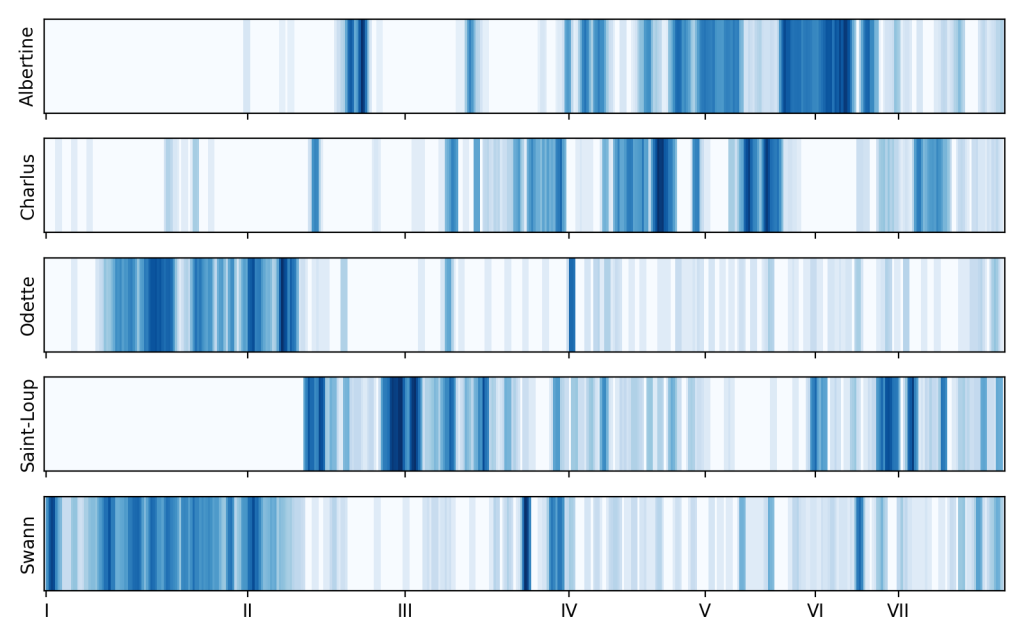
I thought it would be interesting to try and visualize these transitions, so I recorded the chapter and paragraph of each reference of each character, in effect producing “coordinates” for every portion ofthe text. For example, the first proper name in the text (appropriately, François Ier), is (1, 1). I counted the number of references for each name within each of the 486 chapters.

These counts constitute a kind of “character heat map”: when characters are referenced frequently in a chapter, these counts are high, and are zero if a character is not mentioned at all.

I created the following heat map of the top five characters by ripping off some stuff I read on stackoverflow:

The tick marks represent the seven volumes of ISLT and each slender vertical line represents a chapter. Of course, not all chapters are the same length so the diagram is not accurate in that respect. From this visualization you can see the following:

• Albertine does enter the picture in volume II and dominates volumes V and VI;
• Odette features heavily in Volume I (especially in “Swann in Love”), with only intermittent appearances thereafter;
• Saint-Loup is introduced in Volume II and taking over the focus from the Swann-Odette relationship in Volume I;
• Swann is a central figure in Volume I and has occasional reappearances thereafter. When he enters the story he is typically a central figure.

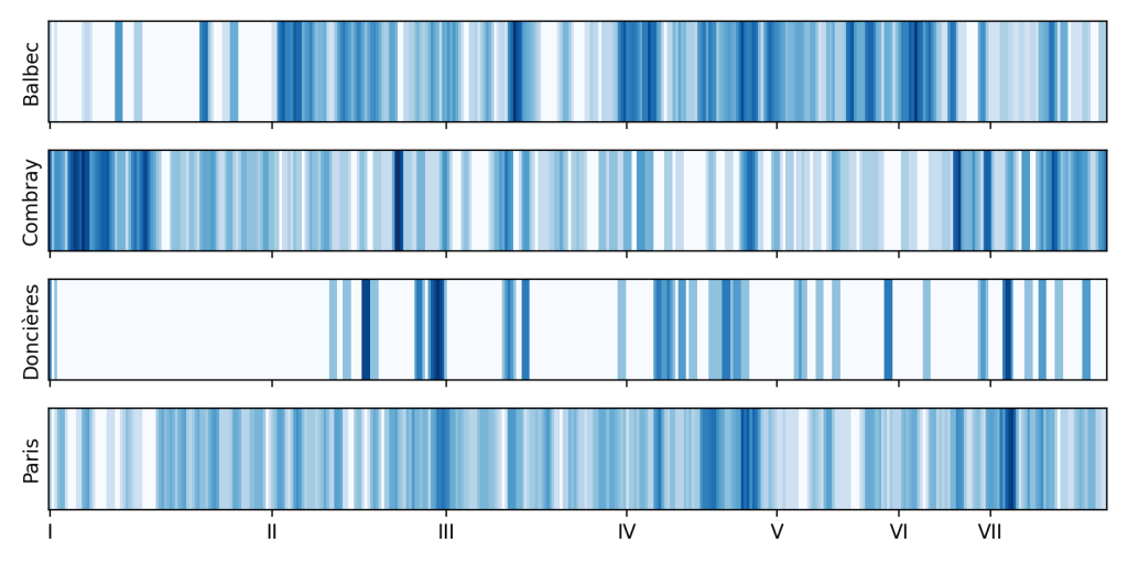
Proust treats places as characters of their own, so it’s also interesting to examine where places are referenced. Here are four frequently referenced places. Combray is where the story starts, of course, whereas Balbec later becomes a place of relaxation and refuge to which Proust returns repeatedly. Doncières is where Saint-Loup (an aspiring officer) is stationed, and so references to Doncières are correlated to those of Saint-Loup. Paris, the beating heart of society, is mentioned throughout ISLT.

I also produced heat maps of five of the most frequently occurring words (each a theme):

There are other ways to visualize and juxtapose references to characters, places, and concepts, of course, and perhaps in future posts I will explore further.

For the next post in this series, however, we will examine the context in which characters are mentioned. Which are referred to in positive and negative terms, and when do changes in sentiment occur?

Advertisement

Names and Places in Proust’s In Search of Lost Time

This post is a continuation of a series where I use natural language processing (NLP) to analyze the text of Proust’s In Search Of Lost Time (ISLT). Here is the Python code for this series.

In my previous post I examined which words most frequently occur in ISLT. You may have noticed that both “faire” and “faisait” – variations of the verb “to do” – appear in the list. If we group variations of the same root word together (for example in English, “am”, “are”, and “was” all group with “be”), then we end up with a better characterization of word frequency. This process is called lemmatization. Lemmatizing reduces the number of unique words in ISLT from 38,662 to 20,948.

The table below summarizes word frequencies for this reduced set. Verbs are dominant: “to do” and “to have” on top, closely followed by “to see”, “to be”, “to know”, “to come”, “to take”, “to say”, “to go”, and “to want”.

faire	5669
avoir	4790
y	3759
voir	3506
être	3307
savoir	2661
venir	2605
dire	2406
aller	2398
vouloir	2378
Albertine	2339
croire	2162
jour	2124
femme	2028
chose	2022
grand	2012
pouvoir	1988
connaître	1934
donner	1856
petit	1827

Twenty most frequently occurring lemmatized words in ISLT

But we should pivot from verbs, shouldn’t we? After all, names and places are of deeper interest to the Narrator of ISLT; in fact the third part of Swann’s Way is called “Place Names: The Name”.

Which names and places are most referenced in ISLT? Using spaCy, I was able to determine the answer. Here are the top 30 names:

Albertine	2338
Swann	1338
Charlus	1303
Saint-Loup	1091
Odette	971
Mme de Guermantes	897
Françoise	787
Gilberte	715
Mme Verdurin	660
Morel	558
Bloch	474
Andrée	383
Mme de Villeparisis	375
duc de Guermantes	328
Brichot	309
Bergotte	300
Norpois	293
Cottard	282
Monsieur	223
Jupien	221
Verdurin	202
Mme de Cambremer	182
Elstir	179
Rachel	168
Vinteuil	167
M. Verdurin	158
Legrandin	154
les Verdurin	137
Mlle Vinteuil	136
Forcheville	118

The 30 most frequently referenced names in ISLT

There are certain to be some errors in these counts, but I gave it a shot. I tried to combine references to different names for the same individual, for example “Robert” and “Saint-Loup” for Saint-Loup, “Mme Swann” and “Odette” for Odette, “Basin” for duc de Guermantes, and so on. Perhaps in the future I will revise this table slightly as I add to my list of aliases.

I will leave deeper analysis to others, but there are two obvious points worth making. The first is that characters are not always referenced by their proper names. Often definite pronouns such as “you”, “him”, “her”, etc are often used in the text. This analysis fails to account for that fact. To do so, I’d need to trace the reference of each definite pronoun back to its source, which I don’t know how to easily do. (I do know that if I did, the most referenced character in ISLT would be, of course, the narrator Marcel – who is mentioned by name only five times, twice in the second paragraph of chapter 345 and three times in the second paragraph of chapter 356, but as “je” countless times.)

Secondly, in my view, the list itself does reflect the true importance of each character within ISLT. For example, Gilberte is quite a critical figure in ISLT, linking the first volume to the last, and symbolizing the theme of regaining time…however she barely makes the top 10 in terms of frequency. Are there better ways of trying to capture the “deeper significance” of characters within a story? Perhaps a future post will revisit this topic.

Moving on, here are the ten most mentioned places:

Balbec	737
Guermantes	657
Paris	521
Combray	426
France	154
Venise	128
Élysées	111
Champs	97
Méséglise	75
Doncières	66

The ten most frequently mentioned places in ISLT

(It seems weird that Champs and Élysées are not recognized by spaCy as belonging to a single compound token; I need to look into the details on that.)

In my next post, I will further examine the use of names and places in ISLT.

Text Analytics on Proust’s In Search of Lost Time

Seven years ago I analyzed the text of Marcel Proust’s In Search of Lost Time to find the five longest sentences (in English). This is the first of a series of posts where I use natural language processing (NLP) to analyze the text of Proust’s sprawling, introspective, and intensely human epic.

The Python code supporting this analysis is provided here. I make frequent use of the popular NLP package spaCy in my code. Unlike my previous Proust posts, here I use the original public domain French text as provided by marcel-proust.com.

The complete text of In Search of Lost Time (ISLT) is comprised of seven volumes consisting of 486 chapters. Including chapter titles there are 6,023,707 characters, including punctuation. There are 1,175,999 words in all, and 38,662 unique words. (The average adult English language vocabulary is 20,000-35,000 words.)

Here the five most used words, with their frequencies. They are boring:

de	52378
la	28637
à	27597
que	25687
et	25238

The five most frequently used words in ISLT

This is not really what we want, of course; it’s just a bunch of conjunctions, articles, and prepositions – all examples of what the NLP world calls “stop words“. The list of most common words changes significantly when we exclude spaCy’s list of French stop words. The results are given below. Even in a simple analysis such as this, some of ISLT’s key themes emerge: place, time, women, men, Albertine, Swann.

y	3759
faire	2868
Albertine	2338
eût	2038
fois	1727
vie	1724
jamais	1643
temps	1632
voir	1570
air	1458
femme	1397
moment	1363
jour	1362
Swann	1337
Charlus	1302
monde	1291
faisait	1249
chose	1246
homme	1033
yeux	1028

The twenty most frequently occurring words in ISLT, excluding stopwords

Word frequency changes in interesting ways. Here is a plot of the 200 most frequent words; a visual representation of my first table. You can see that the frequency drops off quickly from over 50,000 to under 1,000 quickly, followed by a long tail of seldom-used words:

Frequency plot of the 200 most-used words in ISLT

If I exclude stop words, I get a similar result. The curve seems to fit a power distribution reasonably well.

Frequency plot of the 200 most-used words in ISLT, excluding stop words

In the plot above, the most frequent word “y” has rank 1, the next most frequent word “faire” has rank 2, and so on. It is has been observed that the rank and frequency of words in a large corpus of text often follow’s Zipf’s law. Another interesting writeup of Zipf’s law can be found here.

If we plot the log of the rank and the log of the frequency, Zipf’s law says that the result should be linear. When we do this for all 30,000+ unique words in ISLT, we do see something that roughly follows Zipf’s law:

I don’t know what it means, or if it means anything at all…but it’s interesting.

This is just a start. In future posts I will explore references to characters and places within ISLT, and share some interesting findings.

A Lazier Way to Solve Knuth’s Skeleton Multiplication Puzzle

Last time, I described a solution to the following “skeleton multiplication puzzle” from Don Knuth’s The Art of Computer Programming:

        N N N  (1)
    x N N N N  (2)
    ---------  
      N N N 7  (3)
    N N N N    (4)
  N N N N      (5)
  N N N        (6)
  -----------  
  7 7 7 7 7 7  (N != 7)

The answer found by Knuth is the following:

        5 3 9  (1)
    x 1 4 4 3  (2)
    ---------  
      1 6 1 7  (3)
    2 1 5 6    (4)
  2 1 5 6      (5)
  5 3 9        (6)
  -----------  
  7 7 7 7 7 7 

I was able to find a second solution where there was a leading zero in row (4). To find it, I considered all the prime factors of 777777 and reasoned about which pairs could fit the pattern of the puzzle.

In this post I want to show you how I originally found this solution.

I wrote a bit of code in Python to express part of the problem as a constraint programming (CSP) model. Instead of trying to work out the solution myself, I write down the conditions that must be true, and let the constraint programming solver do the work.

The basic approach for solving a puzzle using a solver is:

1. Write down the variables (unknowns) that I want the solver to find.
2. Write down all of the constraints (logical conditions) that need to be true.
3. Turn the above into the right API calls for the solver I am using.

Here’s how it works (and here’s a link to my code). I used the python_constraint package as my CSP solver. To specify the puzzle we need a Problem() object:

problem = Problem()

In a CSP I first define variables that I want the solver to find. The variables I care most about are n_1 and n_2. I know that n_1 < 1000 and n_2 < 10000. addVariable‘s first argument is the name of the variable and the second is the domain.

problem.addVariable("n_1", list(range(100, 999+1)))
problem.addVariable("n_2", list(range(1000, 9999+1))) 

I also am interested in the digits of each number. I will call the digits for the first (d_11, d_12, d_13), and the second (d_21, d_22, d_23, d_24). Remember that none of these digits can be a seven.

not_seven = [0, 1, 2, 3, 4, 5, 6, 8, 9] # no sevens allowed!                

# n_1 = d_13 d_12 d_11                                                      
problem.addVariable("d_13", not_seven)
problem.addVariable("d_12", not_seven)
problem.addVariable("d_11", not_seven)
 
# n_2 = d_24 d_23 d_22 d_21                                                 
problem.addVariable("d_24", not_seven)
problem.addVariable("d_23", not_seven)
problem.addVariable("d_22", not_seven)
problem.addVariable("d_21", not_seven) 

Now I start writing down conditions that I know to be true. The first is that the product is a bunch of sevens:

problem.addConstraint(lambda n_1, n_2: n_1 * n_2 == 777777, ['n_1', 'n_2'])

Even if you know Python this may be confusing because you may not be familiar with the python_constraint package. The point is that I am providing an anonymous (lambda) function that evaluates the product of n_1 and n_2 as the first argument, and the names of the variables I defined earlier as the second.

Next, if I put the digits d_1x together, I get n_1:

problem.addConstraint(lambda d_11, d_12, d_13, n_1:
                      100 * d_13 + 10 * d_12 + d_11 == n_0,
                      ['d_11', 'd_12', 'd_13', 'n_1'])

Same for n_2:

problem.addConstraint(lambda d_21, d_22, d_23, d_24, n_2:
                      1000 * d_24 + 100 * d_23 + 10 * d_22 + d_21 == n_2,
                      ['d_21', 'd_22', 'd_23', 'd_24', 'n_2']) 

Also, as considered earlier, when I multiply the last two digits of n_1 and n_2, the result must end in 7:

problem.addConstraint(lambda d_11, d_21: (d_11 * d_21) % 10 == 7, ['d_11', 'd_21'])

Now, if I wanted to be complete, I would write down a bunch more conditions for all of the Xs that appear in rows 3-6, using the rules of long multiplication. But why would I want to do that? The point is to be lazy.

Let’s just solve the problem, ask for all the solutions, and print them out.

s = problem.getSolutions()
# s is a list of solutions. Each solution is a dict of variable values.     
     for t in s:
         print(f"{t['n_0']} x {t['n_1']} = {t['n_0'] * t['n_1']}") 

Wow! The same four that I discovered above. This was “easier” for me in the sense that I already knew how to use the python_constraint package, so I could just do the coding above without having to “think”. Doing it “the old fashioned way” was in the end more fun, but requires more deliberation and focus for me.

A Skeleton Multiplication Puzzle by Knuth

I want to share with you two ways to solve an interesting puzzle from Don Knuth’s “The Art of Computer Programming“. Here is the first!

The puzzle that caught my attention, quite by chance, is the “skeleton multiplication puzzle” given in Exercise 50 of Pre-Fascicle 9b (called “A Potpourri of Puzzles”). We want to find two numbers whose product is 777777, but we are given very little information. Here is the puzzle:

        N N N  (1)
    x N N N N  (2)
    ---------  
      N N N 7  (3)
    N N N N    (4)
  N N N N      (5)
  N N N        (6)
  -----------  
  7 7 7 7 7 7  (N != 7)

All of the “Ns” are unknown, and none of them can be a 7. Notice that I’ve numbered the rows (1) – (6) because I am going to obsess about them below.

This doesn’t seem like a lot to go on, does it? I’ll give you some space to think about it, then I will show you Knuth’s solution.

….

OK, here’s what Knuth says:

“The only 3-digit divisors of 777777 = 3 x 7 x 7 x 11 x 13 x 37 that contain no 7s and don’t end in 1 are (143, 259, 429, 539). Their cofactors are (5439, 3003, 1813, 1443). And only 539 x 1443 gives just seven 7s.”

So that settles that, right? Well, not quite. Let’s dig into the details.

Let’s call the number in row (1) n_1, and the number in row (2) n_2. We want n_1 * n_2 = 777777.

Remember (or perhaps learn for the very first time…) that for every positive integer, there is a unique set of primes whose product is that number. This is called the prime factorization of a number.  We can use the prime factorization of 777777 to narrow down the possibilities for n_1 and n_2.

From Wolfram Alpha, we can get the prime factors: (3, 7, 7, 11, 13, 37).

Since n_1 * n_2 = 777777,  the prime factors of n_1 and n_2 also come from this set. Let’s focus on n_1. If I go through all the subsets of (3, 7, 7, 11, 13, 37) whose product has three digits, here’s what I find. Hopefully I didn’t miss any!

7 * 37 = 259
11 * 13 = 143
11 * 37 = 407
13 * 37 = 481
3 * 7 * 7 = 147 
3 * 7 * 11 = 231
3 * 7 * 13 = 273
3 * 11 * 13 = 429
11 * 13 = 143
3 * 7 * 37 = 777
7 * 7 * 11 = 539
7 * 7 * 13 = 637

But remember that N != 7, so that means:

• n_1 can’t have a 7 as a digit
• The last number of n_1 cannot be 1, otherwise the last digit of n_2 would be 7, because the last digit of the product is 7: look at row (3).

So now we’re down to these possibilities:

259 (cofactor is 777777/259=3003)
143 (cofactor 5439)
429 (cofactor 1813)
539 (cofactor 1443)

But a full solution has to avoid 7s in rows (3)-(6). So we need to work out the long multiplication to see which of these possibilities are actually solutions. Go ahead and do that on paper now, or you can cheat here. When you do, you will see that Knuth’s solution using 539 and 1443 does solve the puzzle. Of course it does; he’s Don Frigging Knuth.

But hang on a moment…what about this?

        4 2 9  (1)
    x 1 8 1 3  (2)
    ---------  
      1 2 8 7  (3)
    0 4 2 9    (4)
  3 4 3 2      (5)
  4 2 9        (6)
  -----------  
  7 7 7 7 7 7  

Hey, this works too! This new solution is a bit strange because it has a leading zero in row (4), but nobody said I can’t do that. When I wrote Prof. Knuth, he agreed.

There is one more plot twist. It turns out that what I have written here is *not* the way I discovered this alternate solution; I am far too lazy for that. Instead, I used Python to do the thinking for me. Read more next time!

How I Create Presentation Content

Over the years, I have developed an approach for building content for presentations where a PowerPoint or Google Slides deck is required. Here it is, in case it is helpful to you.

I don’t go through this whole process every single time, however if I have no previous content to draw from, I have adequate time to prepare, and I need to do a good job, this is what I do:

1. Write down bullet points for the following. [15 minutes]

• Who is the audience for the presentation?
• Who else is likely to see the presentation?
• Why do they care about the subject?
• What do I want them to know about the topic? (3-5 things)
• What I hope to accomplish by presenting? (1-3 things)
  • This is what you want, not what the audience wants. e.g. for a project to be funded, to hire more people, to give management confidence in the team’s capabilities.

2. Write a short essay about the topic. [1 hour]

• Make an outline of the main points, based on the above.
• Write a 1-3 page essay based on the outline.
• Assume very little prior knowledge.
• Don’t use jargon.
• Do it quickly and don’t worry about flow or structure. I try to write the essay in less than an hour.

3. Do something else for a day or two.

4. Revise your essay. [30 minutes]

• Read it, without consulting your prior notes.
• Pull out the main points based on your reading (or ask someone else to read it and tell you).
• Think about whether the main points should change, or be reworded.
• Edit the essay as necessary.

5. Make a skeleton for the deck. [30 minutes – 1 hour]

• Make a single slide with the main points as bullets.
• Make a single blank slide for each main point, with the main point as the title
• Ask myself which basic concepts need to be explained, and make one slide for each concept.
  • You will reuse these “concept” slides in future decks.
  • Even if your audience is already familiar with the concept, build the slide anyway. You can put it in the appendix. Most of the time, your audience is not as familiar with basic concepts as you think.
• Think about whether there is a good real world example that makes the point.
• Don’t worry about whether the ordering of slides makes sense.

6. Build slides. [several hours]

• Look at one slide at a time.
• If you have content from previous decks that fits, go ahead and pull it in now, as long as it really does fit.
• Think about the point you want to make on the slide.
  • There should be only one main point.
  • If there is more than one point, break into more than one slide.
  • If you end up with too many slides on one topic, don’t worry about that now.
• Think about a picture, data visualization, or table that might make the point well. Re-use old content if you can. Don’t worry about making the visual content look nice at first.
• Work in whatever order feels comfortable.
• Keep doing this until most of the slides have content.
• Do not do an intro slide or a conclusion slide.

7. Edit slides. [several hours]

• Flip through all of the slides and see if there is a logical story being told.
  • Example: “Situation, Obstacle, Action, Result”
• Move slides to the appendix if they seem extraneous
• Start asking for feedback from people you trust, even before you are done editing
• Think about ‘frequently asked questions’ that might come up. If they are important, put them in the main flow. Otherwise, make a slide in the appendix.
• Now get very picky about wording and presentation:
  • Remove extra words
  • Always use the same terminology for the same concept
  • Spell out all acronyms the first time you use them
  • Use consistent fonts, visual styles, and alignments
  • Format all tables properly
  • Always label the axes of charts, and give all charts meaningful titles
  • Add arrows and short comments for things that require particular emphasis. Lower the cognitive burden on your audience.
  • Here are some more tips from a blog post I wrote seven years ago…
• Make an intro slide last.
• Consider omitting a ‘conclusion’ slide – you often don’t need it.

 

Creating Equation Haikus using Constraint Programming

Bob Bosch pointed out (in a response to Shea Serrano, wonderfully…) that 77 + 123 = 200 is a haiku in English:

Somewhat related. This is a haiku (when read in English): pic.twitter.com/aeTMPPIUxi

— Robert (Bob) Bosch (@baabbaash) September 19, 2019

How many such haikus are there? Well, we can use constraint satisfaction (CSP) to give us an idea (Python code here for the impatient):

A traditional haiku consists of three lines: the first line has five syllables, the second seven, and the last five, for a total of seventeen syllables.

We can write equations that describe our problem. First, let’s define the function s[n] as the number of syllables in the English words for n. For example, s[874] = 7; try saying “eight hundred seventy four” out loud. It’s not that hard in English to compute s[n]; at least, I don’t think I messed it up.

Let’s call A the number in the first line of the haiku, B the second, and C the third. If we want a haiku with the right number of syllables and for the equation it describes to hold, all we need is:

s[A] = 5
1 + s[B] = 7 (since “plus” is one syllable)
2 + s[C] = 5 (since “equals” is two syllables)
A + B = C

If you let A=77, B=123, C=200 as in Bob’s example, you will see the above equations hold.

Using the constraint package in Python, it’s easy to create this model and solve it. Here is the code. A great thing about CSP solvers is that they will not just give you one of the solutions to the model, but all the solutions, at least for cases where A, B, C <= 9999. It turns out there are 279 such haikus, including

eight thousand nineteen
plus nine hundred eighty one
equals nine thousand

and the equally evocative

one hundred fourteen
plus one hundred eighty six
equals three hundred

Of course, this is not the only possible form for an equation haiku. For example, why not:

A
+ B + C
= D

I invite you to modify the code and find other types of equation haikus!

Optimizing 19th Century Typewriters

The long title for this post is: “Optimizing 19th Century Typewriters using 20th Century Code in the 21st Century”.

Patrick Honner recently shared Hardmath123’s wonderful article “Tuning a Typewriter“. In it, Hardmath123 explores finding the best way to order the letters A-Z on an old and peculiar typewriter. Rather than having a key for each letter as in a modern keyboard, the letters are laid out on a horizontal strip. You shift the strip left or right to find the letter you want, then press a key to enter it:

What’s the best way to arrange the letters on the strip? You probably want to do it in such a way that you have to shift left and right as little as possible. If consecutive letters in the words you’re typing are close together on the strip, you will minimize shifting and type faster.

The author’s approach is to:

• Come up with an initial ordering at random,
• Compute the cost of the arrangement by counting how many shifts it takes to type out three well-known books,
• Try to find two letters that when you swap them results in a lower cost,
• Swap them and repeat until you can no longer find an improving swap.

This is a strong approach that leads to the same locally optimal arrangements, even when you start from very different initial orderings. It turns out that this is an instance of a more general optimization problem with an interesting history: quadratic assignment problems. I will explain what those are in a moment.

Each time I want to type a letter, I have to know how far to shift the letter strip. That depends on two factors:

1. The letter that I want to type in next, e.g. if I am trying to type THE and I am on “T”, “H” comes next.
2. The location of the next letter, relative to the current one T. For example, if H is immediately to the left of T, then the location is one shift away.

If I type in a bunch of letters, the total number of shifts can be computed by multiplying two matrices:

• A frequency matrix F. The entry in row R and column C is a count of how often letter R precedes letter C. If I encounter the word “THE” in my test set, then I will add 1 to F(“T”, “H”) and 1 to F(“H”, “E”).
• A distance matrix D. The entry in row X and column Y is the number of shifts between positions X and Y on the letter strip. For example, D(X, X+1) = 1 since position X is next to position X+1.

Since my problem is to assign letters to positions, if I permute the rows and columns of D and multiply this matrix with F, I will get the total number of shifts required. We can easily compute F and D for the typewriter problem:

• To obtain F, we can just count how often one letter follows another and record entries in the 26 x 26 matrix. Here is a heatmap for the matrix using the full Project Gutenberg files for the three test books:

• The distance matrix D is simple: if position 0 is the extreme left of the strip and 25 the extreme right, d_ij = abs(i – j).

The total number of shifts is obtained by summing f_ij * d_p(i),p(j) for all i and j, where letter i is assigned to location p(i).

Our problem boils down to finding a permutation that minimizes this matrix multiplication. Since the cost depends on the product of two matrices, this is referred to as a Quadratic Assignment Problem (QAP). In fact, problems very similar to this one are part of the standard test suite of problems for QAP researchers, called “QAPLIB“. The so-called “bur” problems have similar flow matrices but different distance matrices.

We can use any QAP solution approach we like to try to solve the typewriter problem. Which one should we use? There are two types of approaches:

• Those that lead to provably global optimal solutions,
• Heuristic techniques that often provide good results, but no guarantees on “best”.

QAP is NP-hard, so finding provably optimal solutions is challenging. One approach for finding optimal solutions, called “branch and bound”, boils down to dividing and conquering by making partial assignments, solving less challenging versions of these problems, and pruning away assignments that cannot possibly lead to better solutions. I have written about this topic before. If you like allegories, try this post. If you prefer more details, try my PhD thesis.

The typewriter problem is size 26, which counts as “big” in the world of QAP. Around 20 years ago I wrote a very capable QAP solver, so I recompiled it and ran it on this problem – but didn’t let it finish. I am pretty sure it would take at least a day of CPU time to solve, and perhaps more. It would be interesting to see if someone could find a provably optimal solution!

In the meantime, this still leave us with heuristic approaches. Here are a few possibilities:

• Local optimization (Hardmath123’s approach finds a locally optimal “2-swap”)
• Simulated annealing
• Evolutionary algorithms

I ran a heuristic written by Éric Taillard called FANT (Fast ant system). I was able to re-run his 1998 code on my laptop and within seconds I was able to obtain the same permutation as Hardmath123. By the way, the zero-based permutation is [9, 21, 5, 6, 12, 19, 3, 10, 8, 24, 1, 16, 18, 7, 15, 22, 25, 14, 13, 11, 17, 2, 4, 23, 20, 0] (updated 12/7/2018 – a previous version of this post gave the wrong permutation. Thanks Paul Rubin for spotting the error!)

You can get the data for this problem, as well as a bit of Python code to experiment with, in this git repository.

It’s easy to think up variants to this problem. For example, what about mobile phones? Other languages? Adding punctuation? Gesture-based entry? With QAPs, anything is possible, even if optimality is not practical.

Overview: Reductionism in Art and Brain Science

The subtitle of Eric Kandel’s Reductionism in Art and Brain Science is “Bridging the Two Cultures”. Which cultures? Why bridge them?

Kandel’s two cultures are science and humanities: the physical nature of the universe, and the nature of human experience. His claim is that neither culture understands the other’s methodologies or goals. I can accept this claim, though I have no deep experience with either culture.

The real reason Kandel chose to write a book about art and brain science is that he knows a lot about brain science, a lot about art, and likes to talk about them. The intellectual justification is that the modern versions of art and brain science are reductionist in nature. This commonality suggests that the gap between cultures is narrower than it may first appear.

“Reductionist” is a scary and pretentious word, but all it means is breaking things down into parts. Scientific reductionism seeks to explain a complex phenomenon by examining one of its components on “a more elementary, mechanistic level”. This examination often involves experiments on the edge of our understanding, zeroing in on a single component by controlling for others. Kandel explains that modern art uses methodologies similar to those used by scientists: probing the limits of what can be explained or predicted with existing models of reality. This is so because abstract art (unlike representational art) does not seek to show the world in a familiar, three-dimensional way. It explores relationships between shapes, spaces, colors. This is reductionist:

[de Kooning, Excavation, 1950]

De Kooning applies certain artificial restrictions in this work, permitting other dimensions to run free. It is a kind of experiment.

Another reason for the joint study of art and brain science is that their forms of reductionism are related in a fascinating way: the brain subsystems that we use to form our perceptions of reality are highly activated when appreciating certain kinds of abstract art. Kandel pays special attention to the investigative, experimental work of the New York School. When we understand more about how our brain perceives, Kandel says, we can better appreciate what is captivating and unique about abstract art. This kind of investigation need not be a joy kill, as physicist Richard Feynman explains here.

This leads to Kandel’s examination of the nature of perception. Perception is more than what comes in from the outside. Perception based on visual input alone is incomplete and ambiguous: we must apply additional context in order to make sense of a flawed, jittery two dimensional projection of objects in a three-dimensional world. Our eyes are not enough. It’s long been known that the inverse optics problem can only be solved with additional top-down information (see this Quanta article for more). Top-down information helps me figure out that’s not the Statue of Liberty, it’s just a plastic ornament on the dash. Chalk drawings sometimes fool us nonetheless:

Just as perception is incomplete without top-down information, so is art. Art is incomplete without the perceptual and emotional involvement of the viewer (sayeth Riegl). Gombrich calls this the “beholder’s share“: the viewer’s interpretation of what is seen in personal terms. The beholder’s share is what supplies meaning to the picture. It reflects our consciousness and humanity.

As Kandel explains and is widely known, our brain has both top-down and bottom-up processing systems. Bottom-up systems build up higher level conclusions from small pieces of data: three edges joined make a triangle. In the case of visual processing, top-down and bottom-up systems work together to process images, allowing us to interpret the information they contain. Here is a picture:

One of Kandel’s key points is that abstract art relies more heavily on top-down processes than figurative art. Stripping away easily pattern-matched representational images puts more weight on our top-down systems, leaning on our beholder’s share: our imaginations, emotions, and creativity.

That’s quite a bit to digest, yet I’ve summarized only parts of the first four chapters, chapters that provide the motivation for Kandel to dive into topics that clearly provide Kandel joy and intellectual stimulation:

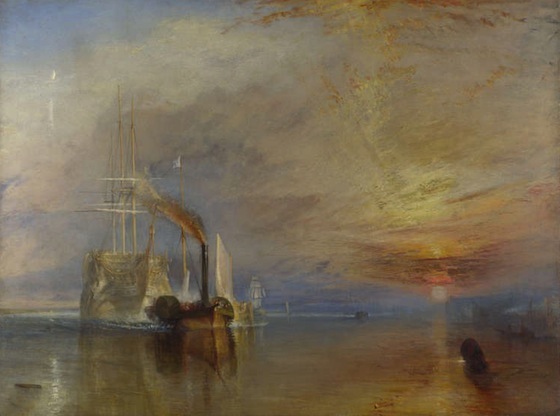
First, the societal and technological change that catalyzed the evolution of Western painting. Oversimplifying: Western painting evolved to depict an increasingly realistic representation of the world (sometimes with help, as chronicled by Hockney and in Tim’s Vermeer) until the advent of photography. Photography can represent reality more accurately than painting, “thus a dialogue emerged through the two art forms”. Painting needed to go elsewhere. A search for an alternative niche began, one of which was greater abstraction. This leads to a discussion of the abstraction of the figurative image by Turner, Mondrian, and others.

Next, investigations of color abstraction,

[Morris Louis, Alpha Pi 1960-1961]

light,
[James Turrell, Meeting]

a return to figuration, reimagined:

[James Katz, Anna Wintour]

and finally the conclusion: that a deeper understanding of brain science will inform and enhance art. It’s fascinating stuff, filled with well-chosen examples.

Kandel provides an entertaining and thoughtful read. In so doing, Kandel takes another step down a path reaching back to the ancient worlds on all continents and through the golden ages of many of the world’s great cultures.

The Origin of CC and BCC

Those born into the computer age unwittingly use metaphors without awareness of their origins. I will explain one such metaphor painfully, and at length: CC.

Before the advent of word processors and personal computers, the typewriter was the dominant tool for producing professional documents. Here is a picture of Robert Caro’s typewriter, the Smith-Corona Electra 210:

An advantage of typewriters is that they can produce legible, consistently formatted documents. A disadvantage is that they do not scale: 1000 copies requires 1000 times the work, unless other accommodations are made. The mass production of a single document was the primary job of the printing press. Later, the mimeograph and the photocopier began to be used in certain schools and organizations. But printing presses, mimeographs, and photocopiers were all expensive.

So along with these more sophisticated tools, there was a simpler, more primal method for document duplication – the carbon copy. Carbon paper, a sheet with bound dry ink on one side, was placed in between two conventional sheets of paper, and the triplet fed into the typewriter. When the keys of the typewriter were struck, the type slug pressed against the ribbon, marking the top page with a character. The slug also pressed against the carbon paper, pressing the dried ink on the back side of the carbon paper onto the second plain sheet of paper, making the same mark. In this way, one key press marked two pages at once. Magic!

Style guidelines for typewritten letters and documents directed authors to indicate when multiple copies of the same document were being distributed to multiple recipients. The notation for this notification was to list the recipients after “cc”, for “carbon copy”.

In other words, an abbreviation for the means of duplication became a notification of duplication.

A variant is the “blind carbon copy“, or BCC. This originally meant carrying out the physical act of duplication – using carbon paper – but omitting the notification. Hence the “blind”: if you are looking at the document, you cannot determine the list of recipients. This carried over to email too.

If you are my age or older, you already knew this. If you are younger, you very likely did not. I was interested in computers in middle school but computer classes were not available. I did the next best thing and took a typing class. That’s how I learned.