Chaining Machine Learning and Optimization Models

Rahul Swamy recently wrote about mixed integer programming and machine learning. I encourage you to go and read his article.

Though Swamy’s article focuses on mixed integer programming (MIP), a specific category of optimization problems for which there is robust, efficient software, his article applies to optimization generally. Optimization is goal seeking; searching for the values of variables that lead to the best outcomes. Optimizers solve for the best variable values.

Swamy describes two relationships between optimization and machine learning:

1. Optimization as a means for doing machine learning,
2. Machine learning as a means for doing optimization.

I want to put forward a third, but we’ll get to that in a moment.

Relationship 1: you can always describe predicting in terms of solving. A typical flow for prediction in ML is

1. Get historical data for:
   1. The thing you want to predict (the outcome).
   2. Things that you believe may influence the predicted variable (“features” or “predictors”).
2. Train a model using the past data.
3. Use the trained model to predict future values of the outcome.

Training a model often means “find model parameters that minimize prediction error in the test set”. Training is solving. Here is a visual representation:

Relationship 2. You can also use ML to optimize. Swami gives several examples of steps in optimization algorithms that can be described using the verbs “predict” or “classify”, so I won’t belabor the point. If the steps in our optimization algorithm are numbered 1, 2, 3, the relationship is like this:

In these two relationships, one verb is used as a subroutine for the other: solving as part of predicting, or predicting as part of solving.

There is a third way in which optimization and ML relate: using the results of machine learning as input data for an optimization model. In other words, ML and optimization are independent operations but chained together sequentially, like this:

My favorite example involves sales forecasting. Sales forecasting is a machine learning problem: predict sales given a set of features (weather, price, coupons, competition, etc). Typically business want to go further than this. They want to take actions that will increase future sales. This leads to the following chain of reasoning:

• If I can reliably predict future sales…
• and I can characterize the relationship between changes in feature values and changes in sales (‘elasticities’)…
• then I can find the set of feature values that will increase sales as much as possible.

The last step is an optimization problem.

But why are we breaking this apart? Why not just stick the machine learning (prediction) step inside the optimization? Why separate them? A couple of reasons:

• If the ML and optimization steps are separate, I can improve or change one without disturbing the other.
• I do not have to do the ML at the same time as I do the optimization.
• I can simplify or approximate the results of the ML model to produce a simpler optimization model, so it can run faster and/or at scale. Put a different way, I want the structure of the ML and optimization models to differ for practical reasons.

In the machine learning world it is common to refer to data pipelines. But ML pipelines can involve models feeding models, too! Chaining ML and optimization like this is often useful, so keep it in mind.

Four Things I Learned from Jack Dongarra

Opening the Washington Post today brought me a Proustian moment: encountering the name of Jack Dongarra. His op-ed on supercomputing involuntarily recalled to mind the dusty smell of the third floor MacLean Hall computer lab, xterm windows, clicking keys, and graphite smudges on spare printouts. Jack doesn’t know it, but he was a big part of my life for a few years in the 90s. I’d like to share some things I learned from him.

I am indebted to Jack. Odds are you are too. Nearly every data scientist on Earth uses Jack’s work every day, and most don’t even know it. Jack is one of the prime movers behind the BLAS and LAPACK numerical libraries, and many more. BLAS (Basic Linear Algebra Subprograms) and LAPACK (Linear Algebra Package) are programming libraries that provide foundational routines for manipulating vectors and matrices. These routines range from the rocks and sticks of addition, subtraction, and scalar multiplication up to finely tuned engines for solving systems of linear equations, factorizing matrices, determining eigenvalues, and so on.

Much of modern data science is built upon these foundations. They are hidden by layers of abstractions, wheels, pips and tarballs, but when you hit bottom, this is what you reach. Much of ancient data science is also built upon them too, including the solvers I wrote as a graduate student when I was first exposed to his work. As important as LAPACK and BLAS are, that’s not the reason I feel compelled to write about Jack. It’s more about how he and his colleagues went about the whole thing. Here are four lessons:

Layering. If you dig into BLAS and LAPACK, you quickly find that the routines are carefully organized. Level 1 routines are the simplest “base” routines, for example adding two vectors. They have no dependencies. Level 2 routines are more complex because they depend on Level 1 routines – for example multiplying a matrix and a vector (because this can be implemented as repeatedly taking the dot product of vectors, a Level 1 operation). Level 3 routines use Level 2 routines, and so on. Of course all of this obvious. But we dipshits rarely do what is obvious, even these days. BLAS and LAPACK not only followed this pattern, they told you they were following this pattern.

I guess I have written enough code to have acquired the habit of thinking this way too. I recall having to rewrite a hilariously complex beast of project scheduling routines when I worked for Microsoft Project, and I tried to structure my routines exactly in this way. I will spare you the details, but there is no damn way it would have worked had I not strictly planned and mapped out my routines just like Jack did. It worked, we shipped, and I got promoted.

Naming. Fortran seems insane to modern coders, but it is of course awesome. It launched scientific computing as we know it. In the old days there were tight restrictions on Fortran variable names: 1-6 characters from [a-z0-9]. With a large number of routines, how does one choose names that are best for programmer productivity? Jack and team zigged where others might have zagged and chose names with very little connection to English naming.

“All driver and computational routines have names of the form XYYZZZ”

where X represents data type, YY represents type of matrix, and ZZZ is a passing gesture at the operation that is being performed. So SGEMV means “single precision general matrix-vector multiplication”.

This scheme is not “intuitive” in the sense that it is not named GeneralMatrixVectorMultiply or general_matrix_vector_multiply, but it is predictable. There are no surprises and the naming scheme itself is explicitly documented. Developers of new routines have very clear guidance on how to extend the library. In my career I have learned that all surprises are bad, so sensible naming counts for a lot. I have noticed that engineers whom I respect also think hard about naming schemes.

Documentation. BLAS and LAPACK have always had comprehensive documentation. Every parameter of every routine is documented, the semantics of the routine are made clear, and “things you should know” are called out. This has set a standard that high quality libraries (such as the tidyverse and Keras – mostly) have carried forward, extending this proud and helpful tradition.

Pride in workmanship. I can’t point to a single website or routine as proof, but the pride in workmanship in the Netlib has always shone through. It was in some sense a labor of love. This pride makes me happy, because I appreciate good work, and I aspire to good work. As a wise man once said:

Once a job is first begun,
Never leave it ’till it’s done.
Be the job great or small,
Do it right or not at all.

Jack Dongarra has done it right. That’s worth emulating. Read more about him here [pdf] and here.

2018 NCAA Tournament Picks

Every year since 2010 I have used data science to predict the results of the NCAA Men’s Basketball Tournament. In this post I will describe the methodology that I used to create my picks (full bracket here). The model has Virginia, Michigan, Villanova, and Michigan State in the Final Four with Virginia defeating Villanova in the championship game:

Here are my ground rules:

• The picks should not be embarrassingly bad.
• I shall spend no more than one work day on this activity (and 30 minutes for this post). This year I spent two hours cleaning up and running my code from last year.
• I will share my code and raw data. (The data is available on Kaggle. The code is not cleaned up but here it is anyway.)

I used a combination of game-by-game results and team metrics from 2003-2017 to build the features in my model. Here is a summary:

• Team features
  • Massey ratings, obtained here.
  • My own eigenvalue centrality model, which tends to do a good job all by itself.
  • Metrics from Ken Pomeroy’s page. (These are public and are therefore fair game.)
  • Dean Oliver’s “Four Factors”, which I calculate from per-game data.
• Game features
  • Home court. (1 = home, -1 = away, 0 = neutral)
  • Year
  • (I did not have time to use site locations – the code is buggy.)

I also performed some post-processing:

• I transformed team ranks to continuous variables given a heuristic created by Jeff Sonos.
• Standard normalization.
• One hot encoding of categorical features.
• Upset generation. I found the results to be not interesting enough, so I added a post-processing function that looks for games where the win probability for the underdog (a significantly lower seed) is quite close to 0.5. In those cases the model picks the underdog instead.

The model predicts the probability one team defeats another, for all pairs of teams in the tournament. The model is implemented in Python and uses logistic regression. The model usually performs well. Let’s see how it does this year!

Advice for Underqualified Data Scientists

A talented individual seeking entry-level data science roles recently asked me for advice. “How can you show a potential employer that you’d be an asset when on paper your resume doesn’t show what other candidates have?”

I’ll stick to data science, but much of what I share applies to other roles, too.

Let’s think about the question first. Why do coursework and skills matter for employers? It depends. Different employers have different philosophies about how they evaluate candidates. Most job listings specify required skills and qualifications for applicants, for example “must have 3-5 experience programming in R or Python.” Usually there is more to the story. Sometimes employers don’t expect candidates to meet all the criteria. Other times, the criteria are impossible to meet.

In most situations, employers are looking for additional attributes not provided in the job listing. Some employers will tell you their philosophy by listing the attributes they value: “ability to deal with ambiguous situations”, “being a team player”, “putting the customer first”, “seeks big challenges”, and so on. Others don’t. Even if they tell you, you don’t typically know which attributes are most important. What really matters? If I am a so-so programmer but a brilliant statistician, do I have a shot?

Individuals who make hiring decisions have a mental image of how a successful candidate will perform on the job. This mental image includes possessing and using a certain set of skills. Qualifications such as a degree, a certificate, or code on github provide part (but only part) of the evidence necessary to ensure hiring managers that they are making a sound decision.

Let’s be simplistic and say that employers consider both “explicit skills” and “implicit skills”. Examples of explicit skills are demonstrated knowledge or capability with programming language X, technology Y, or methodology Z. Examples of implicit skills might be the ability to break down a complicated problem into its constituent parts, dealing with ambiguity, working collaboratively, and so on. Certainly some employers are very focused on finding candidates with explicit skills, sometimes to the exclusion of implicit skills.

A reframing of the question is then: “If I sense that a potential employer is looking for certain explicit skills and I don’t think I have them, what do I do?” Here are some ideas:

Provide evidence you are good at acquiring explicit skills. Given an example of learning an explicit skill. (“No, I don’t know R, but I know Python. In my blah blah class I had to learn Python so I could apply it to XYZ problem, and it was no big deal. I did ABC and now my code is up on github. Learning R is really not a big deal, I’m confident I could hit the ground running. What would you have in mind for me for my first project?”)

Emphasize your implicit skills. Game plan about questions you’ll be asked and think about how you’d highlight what you believe to be your differentiating skills. (Without sounding like a politician.) By the way, now that I think about it, I followed my own advice when I interviewed at Market6 (now 84.51). I talked about the fact that I have worked in both software engineering and data science roles, and that made me uniquely qualified to work at a company that was trying to deliver data science at scale through SaaS offerings.

Do your own screening. Focus your search on employers who seem to value implicit skills. Rule out others. Do your research prior to applying. Ask friends or contacts. Early in your conversations with employers you can ask the recruiter about their philosophy. Not every job is right for you, so try and figure out which ones are.

That’s all I’ve got. I will close by telling two quick stories.

First story: My first job after finishing my PhD was as an entry level software engineer at Microsoft. When I interviewed, I was fortunate because Microsoft weighted implicit skills highly in their evaluation process. One of my favorite bosses at Microsoft was a classics major (as in Euripides, not the Stones). Another engineering manager started his career localizing dialog box messages into French. Oui, c’est vrai. Both had, and continue to have, a very strong set of implicit skills. They, in turn, looked for implicit skills. Talent comes in many different packages.

Second story: I believe that for early career stage positions it’s important to weight implicit skills more highly than explicit ones. Sometimes it’s a relief if certain explicit skills aren’t there! Several years ago, I had an entry level scientific researcher on my team who did not know how to code, in a position where lots of coding was required. This individual had very deep knowledge of optimization and statistics, was a hard worker, and was incredibly motivated. I was thrilled that they didn’t know how to code because then I could teach them! No bad habits!

 

Two Frustrations With the Data Science Industry

I saw some serious BS about data science on LinkedIn last night. This is nothing new, but this time I couldn’t help myself. I went on a small rant:

I don’t give a shit if you call yourself a data scientist, an analyst, a machine learning practitioner, an operations research specialist, a data engineer, a modeler, a statistician, a code poet, or a squirrel. I don’t care if you have a PhD, if you went to MIT or a community college, if you were born on a farm or in a city, or if Andrew Ng DMs you for tips. I want to know what you can do, if you can share, if you can learn, if you can listen, and if you can stand for what is right even if it’s unpopular. If we’re good there, the rest we can figure out together.

I must have tapped into something, so I’d like to myself a bit more thoroughly.

My rant is rooted in two frustrations about data science.

My first frustration relates to overclassification. How many different terms can we use to refer to data scientists? I honestly don’t know. I have it on authority that there are six types of data scientists. No, wait, there are seven. Strike that, eight. Actually there are ten. Stop the insanity!

The industry itself is also subject to this kind of sillified stratification. I don’t know what the hell I do anymore. Is it operations research? Statistics? Analytics? Machine Learning? Artificial Intelligence? All of it? It depends which thought leadership piece I read. And what is the current state of this field, anyway? Are we in the age of Analytics 2.0? Or is it 3.0? Is big data saving the world, or is it the “trough of disillusionment”? I find all of this unhelpful.

Why is this happening? The use of computer models to learn from data has been around for at least five decades now, but data science has moved from an unnamed, specialized backwater into a rapidly growing and vital industry. This growth has created a market for teaching others about this hot new field. It has also led to the organization of a hierarchy of those who are “in the know” and those who are not. These are the factors driving the accelerating creation of labels and classifications.

However, knowing the names of things does not constitute understanding of essence; the proliferation of labels under the banner of “thought leadership” is often a gimmick; and as Martin Gardner said, inventing your own terminology is a sign of a crank. Debates about terminology often draw us away from doing good data science. Maybe it’s just me but sometimes I get the feeling these distractions are on purpose. They don’t help anyone solve any problems, that’s for sure.

The second frustration I have is overreliance on credentials. As opposed to academic or research positions, my own work in industry has been focused on the practical use of data science to address business problems. More often than not, I’ve worked as part of a team to get the job done. What matters for people like me is whether problems actually get solved, in a reasonable amount of time with a reasonable amount of expense.

I have encountered situations where employers would only consider applicants who had graduated from certain schools, or with certain degrees, or with a certain number of years of experience with a certain specific technical skill. All of these qualifications are proxies for what actually matters: whether someone can meaningfully contribute to team-based analytical problem solving. Focusing on proxies results in both Type I and Type II errors: hiring scientists with great credentials but an inability to deliver (“all hat and no cattle“), or even worse, missing out on the opportunity to hire the proverbial “unicorn” because they didn’t tick the right box. I’ve seen both happen. These proxies are not without their uses: if I really require the development of an MINLP solver to solve optimization models with a particular structure…the right candidate very likely has a PhD. The point is not to confuse correlation with causation. Having a PhD does not make me a great data scientist. Nor does github, nor Coursera, nor Kaggle points. We need to dig deeper.

I suppose I should end positively. The last part of my rant was an appeal to inclusiveness and an appeal to pragmatism. Practical data science means making tradeoffs, large and small, every single day. It means seeing the big picture but also being willing to dig into the details. Let’s take this same practical mindset in growing our skills and building our teams.

Forecasting iPad Sales using Facebook’s Prophet

The past couple of days I’ve been playing around with Facebook’s Prophet, a time series forecasting package.

I used Prophet to forecast quarterly sales of the Apple iPad, all in about 30 lines of Python. The repository for my code is here, and here’s a Jupyter notebook that walks through how it works.

It’s a lot of fun, and you get nice little visualizations like this one:

Check it out!

 

2017 NCAA Tournament Picks

Every year since 2010 I have used analytics to predict the results of the NCAA Men’s Basketball Tournament. I missed the boat on posting the model prior to the start of this year’s tournament. However, I did build and run a model, and I did submit picks based on the results. Here are my model’s picks – as I write this (before the Final Four) these picks are better than 88% of those submitted to ESPN.

Here are the ground rules I set for myself:

• The picks should not be embarrassingly bad.
• I shall spend no more than one work day on this activity (and 30 minutes for this post).
• I will share my code and raw data. (Here it is.)

I used a combination of game-by-game results and team metrics from 2003-2016 to build the features in my model. Here is a summary:

• Team features
  • Massey ratings which I obtained here.
  • My own eigenvalue centrality model, which tends to do a good job all by itself.
  • Metrics from Ken Pomeroy’s page. (These are public and are therefore fair game.)
  • Dean Oliver’s “Four Factors”
• Game features
  • Home court. (1 = home, -1 = away, 0 = neutral)
  • Year
  • (I had ‘day of season’ in there but pulled it. This is implicitly accounted for in some the team features above.)

I also performed some post-processing:

• I transformed team ranks to continuous variables given a heuristic created by Jeff Sonos.
• Standard normalization.
• One hot encoding of categorical features.
• Upset generation. I found the results aesthetically displeasing for bracket purposes, so I added a post-processing function that looks for games between Davids and Goliaths (i.e. I compare seeds) where David and Goliath are relatively close in strength. For those games, I go with David.

I submitted the model to the Kaggle NCAA competition, which asks for win probabilities for all possible tourney games, where submissions are scored by evaluating the log-loss of actual results and predictions. This naturally suggests logistic regression, which I used. I also built a fancy pants neural network model using Keras (which means to run my code you’ll need to get TensorFlow and Keras in addition to the usual Anaconda packages). Keras produces slightly better results in the log-loss sense. Both models predict something like 78% of past NCAA tournament games correctly.

There are a couple of obvious problems with the model:

• I did not actually train the model on past tournaments, only on regular season games. That’s just because I didn’t take the time.
• Not accounting for injuries.
• NCAA games are not purely “neutral site” games because sometimes game sites are closer to one team than another. I have code for this that I will probably use next year.
• I am splitting the difference between trying to create a good Kaggle submission and trying to create a “good” bracket. There are subtle differences between the two but I will spare you the details.

I will create a github repo for this code…sometime. For now, you can look at the code and raw data files here. The code is in ncaa.py.

Noise Reduction Methods for Large-Scale Machine Learning

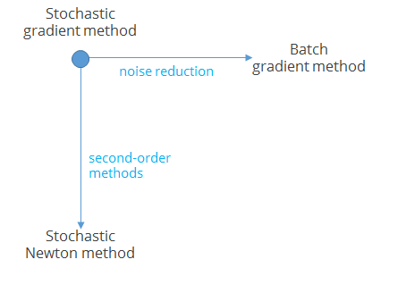
I have two posts remaining in my series on “Optimization Methods for Large-Scale Machine Learning” by Bottou, Curtis, and Nocedal. You can find the entire series here. These last two posts will discuss improvements on the base stochastic gradient method. Below I have reproduced Figure 3.3, which suggests two general approaches. I will cover noise reduction in this post, and second-order methods in the next.

The left-to-right direction on the diagram signifies noise reduction techniques. We say that the SG search direction is “noisy” because it includes information from only one (randomly generated) sample per iteration. We use a noisy direction, of course, because it’s too expensive to use the entire gradient. But we can consider using a small batch of samples per iteration (a “minibatch”), or using information from previous iterations. The idea here is to find a happy medium between the far left of the diagram, which represents one sample per iteration, and the right, which represents using the full gradient.

Section 5 describes several noise reduction techniques. Dynamic sample size methods vary the number of samples in a minibatch per iteration, for example by increasing the batch size geometrically with the iteration count. Gradient aggregation, as the name suggests, involves the use of gradient information from past iterations. The SVRG method involves starting with a full batch gradient, then for subsequent iterations updating the gradient using gradient information at a single sample. The SAGA method involves “taking the average of stochastic gradients evaluated at previous iterates”. Finally, iterate averaging methods use the iterates from multiple previous steps to update the current iterate.

The motivations behind these various noise reduction methods are more or less the same: make more progress on a single step without paying too much of a computational cost. The primary tradeoff, in addition to increased computational cost per iteration, of course, is the extra storage associated with keeping extra state to compute search direction. Section 5 of the paper discusses these tradeoffs in light of convergence criteria.

[Updated 8/24/2016] Going back to our diagram, the up and down dimension of the diagram represents so-called “second-order methods”. Gradient-based methods, including SG, are first-order methods because they use a first-order (linear) approximation to the objective function we want to optimize. Second-order methods attempt to look at the curvature of the objective function to obtain better search directions. Once again, there is a tradeoff: using the curvature is more work, but we hope that by computing better search directions we’ll need far fewer iterations to get a good solution. I had originally intended on covering Section 6 of the paper, which describes several such methods in detail, but I will leave the interested reader to dig through that section themselves!

Analyses of Stochastic Gradient Methods

I am continuing my series on “Optimization Methods for Large-Scale Machine Learning” by Bottou, Curtis, and Nocedal. You can find the entire series here.

Last time we discussed stochastic and batch methods for optimization in machine learning. In both cases we’re trying to optimize a loss function that will give us good learning parameters for a deep learning model. We do this iteratively. A pure stochastic gradient (SG) approach picks one sample per iteration to define a search direction, whereas a batch method will pick multiple samples.

In this post I want to cover most of Section 4, which concerns the convergence and complexity of SG methods. For completeness I have reproduced the authors’ summary of a general purpose SG algorithm below:

Choose an iterate w_1
for k = 1, 2, … do
   generate a random number s_k
   compute a stochastic vector g(w_k, s_k)
   choose a stepsize a_k > 0.
   w_k+1 <- w_k – a_k g(w_k, s_k)

In this algorithm, g is the search direction. In this series, we’ve already discussed three different choices for g:

• g is the gradient. This is conventional gradient descent. In this case the random number is ignored.
• g is the gradient for a single sample. This is conventional stochastic gradient.
• g is the gradient over a subset of the samples. This is “mini-batch” SG.

As the authors show, it’s not easy to make definitive statements on comparison between mini batch and SG. The gist of what they show is that SG has better convergence properties in theory, but batch methods can provide certain practical advantages. That is: “one can, however, realize benefits of mini-batching in practice since it offers important opportunities for software optimization and parallelization; e.g., using sizeable mini-batches is often the only way to fully leverage a GPU processor.” The rest of Section 4 spells this out in more detail through convergence results and complexity analysis.

As a practitioner, I honestly don’t place huge weight on the convergence theorems presented in Section 4. The key result for me is Theorem 4.9, which states that for a nonconvex objective (which we have in most deep learning scenarios) the SG method converges when the stepsize diminishes according to a somewhat loosely defined schedule.

More interesting (for me) is Section 4.4, which discusses the overall work complexity for applying SG to deep learning scenarios. In many real-world big data scenarios, we’re optimizing a loss function using previously trained model parameters under a particular computational time limit. This is different from many traditional optimization scenarios, where we let the code run until we achieve a particular solution accuracy. In our situation, the total expected error in the model is the sum of three components: the expected risk using optimal parameters, the estimated error in the expected and empirical risk, and the optimization accuracy. Minimizing this error involves tradeoffs, for example “if one decides to make the optimization more accurate … one might need to make up for the additional computing time by: (i) reducing the sample size n, potentially increasing the estimation error; or (ii) simplifying the function family H, potentially increasing the approximation error.” These are familiar techniques for machine learning practitioners; the benefit provided here is a more formal characterization of how these techniques impact the overall solution error.

Returning to the choice of conventional versus batch approaches, the discussion in Section 4.5 shows that “Even though a batch approach possesses a better dependency on epsilon, this advantage does not make up for its dependence on n. […] In conclusion, we have found that a stochastic optimization algorithm performs better in terms of expected error, and, hence, makes a better learning algorithm in the sense considered here.” Again, even this statement could be mitigated somewhat by the computational benefits associated with batching on a particular computational infrastructure, that is, the benefits of GPUs and parallelism.

Section 4.5 is a commentary on some of the remaining challenges and questions that must be confronted when using SG for large-scale machine learning. Since the issues raised in Section 4.5 pair nicely with the discussion in Section 5, I’ll save both for next time.

Stochastic and Batch Methods for Machine Learning

I am continuing my series on “Optimization Methods for Large-Scale Machine Learning” by Bottou, Curtis, and Nocedal. You can find the entire series here.

In previous posts we discussed the use of deep neural networks (DNNs) in machine learning, and the pivotal role of the optimization of carefully selected prediction functions in training such models. These topics roughly correspond to the first two sections of the paper.

Section 3 provides an overview of optimization methods appropriate for DNNs. We begin where we left off in Section 2 by assuming a family of prediction functions parameterized by w. In other words, w represents the learning parameters. We also assume a loss function that depends on predicted and actual values, for example misclassification rate. Typically we’re minimizing the loss function f over a set of samples – the empirical risk. We call this R_n(w), which in turn is the average of the loss for each sample: (1/n) Ʃ_i∇f_i(). Given all of this, there are two fundamental paths for minimizing risk. In each case we iteratively improve the learning parameters step by step, where we write the parameters at step k as w_k.

• stochastic: w_k+1 ← w_k − α_k ∇f_ik (w_k) where the index ik is chosen randomly.
• batch: w_k+1 ← w_k − (α_k / n) Ʃ_i∇f_i(w_k)

The difference between the two paths is how many samples we consider on each step. The tradeoff is between per iteration cost (where stochastic wins) versus per iteration improvement (where batch wins). Stochastic algorithms a good choice for DNNs because they employ information more efficiently. If training samples are the same, or similar, than the added value of per step improvement from batch is not going to be worth it, because some (or most) of the added value turns out to be redundant. “If one believes that working with only, say, half of the data in the training set is sufficient to make good predictions on unseen data, then one may argue against working with the entire training set in every optimization iteration. Repeating this argument, working with only a quarter of the training set may be useful at the start, or even with only an eighth of the data, and so on. In this manner, we arrive at motivation for the idea that working with small samples, at least initially, can be quite appealing.”

The authors summarize: “there are intuitive, practical, and theoretical arguments in favor of stochastic over batch approaches in optimization methods for large-scale machine learning”. I will omit a summary of the theoretical motivations, but they are found in Section 3.3.

Next the authors consider improving on SG. One path involves trying to realize the best of both worlds between batch and stochastic methods, namely preserving the low per-iteration cost of stochastic methods while improving the per-iteration improvement. Another path is to “attempt to overcome the adverse effects of high nonlinearity and ill-conditioning”.  This involves trying to employ information beyond just the gradient. We’ll examine these alternatives in future posts in this series, when we get to later sections in the paper.